The Usual(ish) Cylinder Project

In my Junior year of college for a Fluid Dynamics class, we had a lab in a watertunnel that featured a cylinder—introducing me to to the Von-Kármán Vortex Street and how the flow characteristics about an infinite aspect-ratio cylinder change as a function of the Reynolds number $Re$, which is defined by:

where $U$ and $L$ are respectively the flow velocity and geometric characteristic length and $\nu$ is the kinematic viscosity of the fluid.

The Reynolds number effectively governs the proportion of a fluid’s internal forces being driven by inertia compared to viscosity. The classic example comparison is between water and honey, with water having a much larger Reynolds number. Lower reynolds number fluids are dictated by viscous force interactions, which work to dissipate turbulence in the fluid—restricting vorticity, which is defined by:

Where $\omega$ corresponds to a fluid’s capacity to rotate (swirl).

The vortex street behind a bluff body like an infinite aspect-ratio cylinder (circle in two dimensions) is created when small perturbations to the flow manifest themselves and compound. The mathematical basis for this is given in the incompressible Navier-Stokes equation (neglecting gravity, buoyancy, and body forces):

In other words, when flow moves past a non-streamlined shape such as a circle, small disturbances from the non-linear $(\mathbf{U} \cdot \nabla)\mathbf{U}$ term leades to small changes in pressure which drive changes in velocity. This makes the pressure on one side of the circle slightly different from the other—driving accelerations to the fluid. For low Reynold flows, the $\nu \nabla^2 \mathbf{U}$ term works as a viscous dampener, wanting to prevent flow disturbances (which is why honey can’t be stirred). However, if the Reynolds number increases, the dampening is overcome by the flow’s inertia, in which the non-linear terms function as what we refer to as turbulence.

It is in this regime that the flow begins to show periodic oscillations, as the flow chases low pressure regions, and where the ensuing motion leads to new ones forming. This pattern leads to lower and lower pressure regions and more rapid accelerations to account for the gradients. Yet, the high pressure from the incoming flow clamps the sinusoidal pattern from getting more chaotic, limiting the low pressure regions (center of shed vortices) to be mostly behind the circle, which works to dampen the range of the lift coefficient $C_l$.

Any change in flow turbulence thus changes the characteristics of the vortex street, namely the amplitude and frequency of the vortex shedding. To quantitatively analyze the behavior of the vortex street the non-dimensional Strouhal number is used, denoted as

where $f$ is the vortex shedding frequency. The Strouhal number is implemented to standardize the shedding frequency for a range of flow speeds and cylinder sizes. The aim of the class project was to take a quantitative look into the relationship between the Strouhal number and the Reynolds number.

This was the focus of the report below, which delves more into my new fluid simulation tool of choice (Waterlily.jl) and the relationship between shedding behavior and Reynolds number. For the report, I used Waterlily.jl to take snapshots of the vorticity field at a steady state, while logging a time series of the lift coefficient $C_l$. The results captured the key relationships, and are discussed in the document. It is worth noting that the $C_l$ results are slightly inaccurate. In the Appendix, you’ll note that I used:

function get_forces!(sim,t)
    sim_step!(sim,t,remeasure=false)
    force = WaterLily.pressure_force(sim)
    force./(0.5*sim.L*sim.U^2) # normalize for coefficients
end

This is slightly inaccurate, as last.(forces) later on only pulls the normalized lift coefficient as a result of pressure forces, which neglect viscous forces on the cylinder. This is relatively minor, as the circle’s bluff (non-streamlined) geometry imply that pressure forces dominate. To qualitatively show this, consider a simulation at $Re=120$:

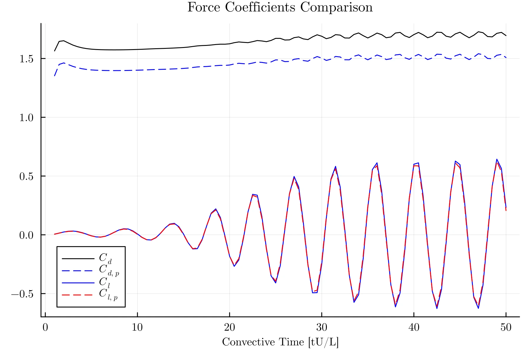
The viscous drag term is worth considering. However, in the report below, I had only considered the lift term, which is relatively unaffected by viscous forces. This is because the viscous force is only influencing lift in the short period of time that it is being deviated from the freestream direction:

$\frac{U_y}{|\vec{U}|}$ is always extremely small, which is why the viscous contribution to lift is fairly negligible.

Ok. So from the perhaps confusing and brief background above, hopefully the following report makes sense:

Note: If you’re checking this out on mobile, the embedded pdf gets a little sluggish. I suggest just clicking the Download Report PDF button.

Despite running into the limitations of Waterlily.jl the academic project was useful, and I quickly found myself wanting to extend slightly. How? Well, I wanted to observe the transient beginning to each case!

Let’s start with lift and drag:

Yeesh. There’s probably a better way to show that information 😊… (might have to click “play” to run the animations and “expand” to see them clearly…additionally, it appears there may be an issue if playing with mobile.)

Nice. It is worth noting that the normalized vortex strength is qualitative, as including the colorbar made the animation appear clunky, however, we can quickly see that the magnitude of the vorticity changes with a change in Reynolds number. WaterLily.jl struggles to resolve the high fidelity effects that differentiate the more turbulent cases. However, if you look closely, you can see that the higher Reynold’s tests have more micro-eddies that are shed. The animations of course buttress the discoveries from the paper. However, I found the transient formation of the vortices helpful when differentiating test cases 😁.

Ultimately, this was a nice short yet comprehensive dive into the Von-Kármán vortex street. I hope the visuals were useful and cool looking!